
SUT30-001
Understanding Complexity Through Disorder

At some point in our lives, we have all heard that systems tend toward disorder. It is one of those ideas that appears almost everywhere: in physics, biology, information, and even in the way we casually talk about life. Ice melts, gases spread, cells lose their organisation after death, and shuffled cards rarely return to order on their own. The destination often seems the same: things move away from neatness, but the path there is rarely smooth or simple.
When we pay attention to the process itself, we notice that systems do not usually become disordered in a simple, featureless way. They form patterns: cream folds into coffee as swirls, gases diffuse through gradients, and materials crack, cluster, separate, and mix before settling into a more uniform state. Somewhere in that movement, complexity appears.
It is a strange observation: as systems move toward disorder, they do not always become less interesting. Somewhere along the way, structure appears. To make sense of this, we begin by first understanding complexity.
An Intuition for Complexity
The movement toward disorder is usually understood through entropy. To see this more clearly, consider a simple example popularised by theoretical physicist Sean Carroll: pouring cream into a cup of black coffee.
In the example, the cream initially sits on top of the coffee, cleanly separated, representing a state of low entropy, or low disorder. As time passes, the liquids begin to diffuse as the system transitions from a low-entropy state to a higher-entropy one. At the point of maximum entropy, the two liquids completely mix, forming a uniform state representing maximum disorder.
The illustration below shows the process unfolding over time. From an entropic point of view, time appears to move in a particular direction; as the liquids diffuse, the system monotonically moves from a rather ordered state to a disordered one.

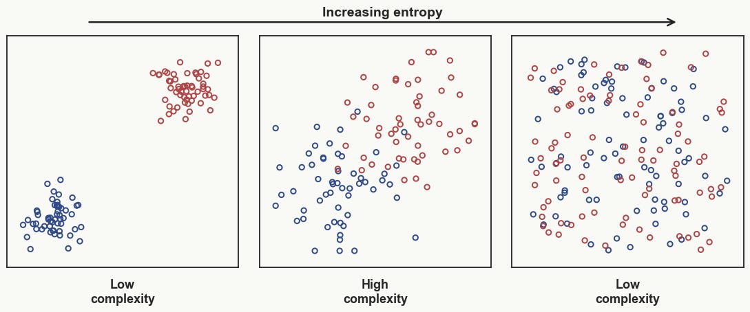
However, when examining the evolving complexity of the process, we notice that in the earlier stages of the system, where entropy is low, we find ourselves with a rather simple configuration: cream and coffee, cleanly separated. As we progress forward, the clear distinction breaks down into a complex pattern, with tendrils of cream penetrating deeper into the settled black coffee and forming a gradient of white, brown, and black.
In the final stages of the process, at maximum entropy, we observe yet another simple configuration: a uniform and boring mixture of coffee and cream. In other words, as entropy increases, complexity first rises, reaches a maximum, and then begins to fall again.
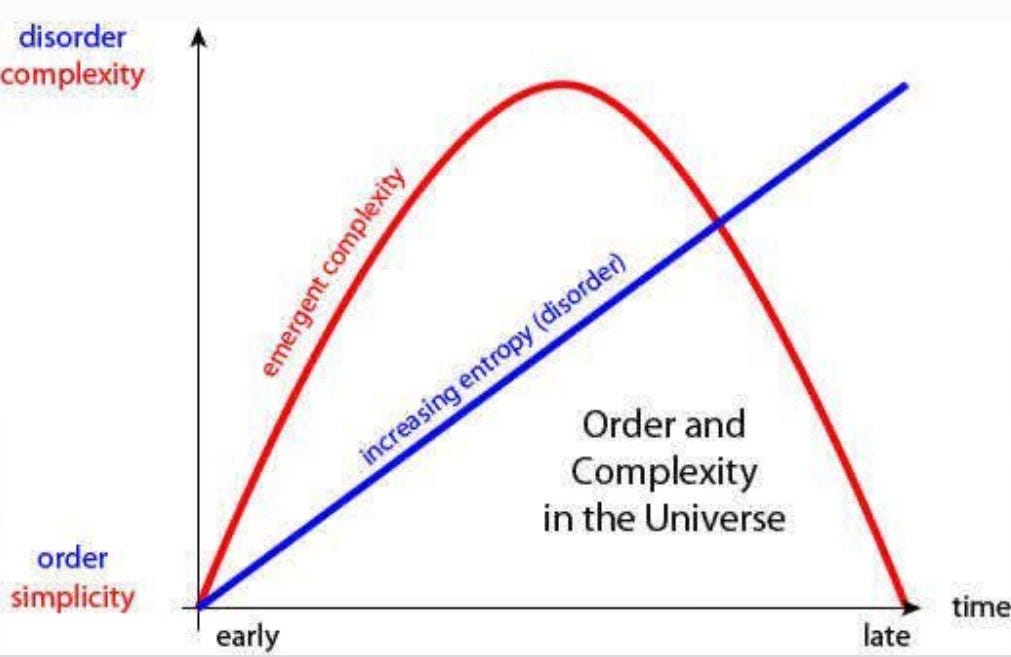
This visual intuition is not limited to coffee and cream. A similar pattern of rising and falling complexity appears in many entropy-driven processes, from physical systems like melting ice to statistical systems like a shuffled deck of cards. In a much looser sense, the same idea is sometimes extended to the universe itself.
To move from intuition to something more precise, we need a way to describe this rise and fall formally. This is where computer scientist Scott Aaronson introduces what he calls the “First Law of Complexodynamics” from his blog post.
A Computational Handle on Complexity
The issue now is that while we can intuitively describe a system's complexity, it is harder to analyse it without linking it to a quantitative measure. In natural language, for example, we could count the number of words spoken, but that would only measure length, not the actual complexity of what was being said. So before jumping into a formal measure, we can first establish a few basic constraints on the kind of complexity we just saw.
Aaronson’s idea begins with the conjecture that complexity in the initial and final phases of an entropic process should be close to zero. The reason is simple: at the beginning of the process, when entropy is lowest, the system is highly ordered, which constrains its complexity and plausibly places an upper bound on it. At the end of the process, the system reaches equilibrium, resembling a uniform state, which also constrains complexity. At intermediate times, neither of these constraints applies, leaving room for complexity to become large.
To understand this rising and falling complexity more precisely, Aaronson turns to Kolmogorov complexity as a computational way of thinking about the information required to describe a system’s state. So far, we have been talking about an intuitive kind of complexity: the kind that rises in the middle of an entropic process and falls again near equilibrium. Aaronson calls this complextropy. Kolmogorov complexity, however, refers to something more specific: the amount of information required to describe a state at a given time. More formally, it is defined as the length of the shortest computer program that can be used to generate a specific piece of data, or, in our case, a specific state.
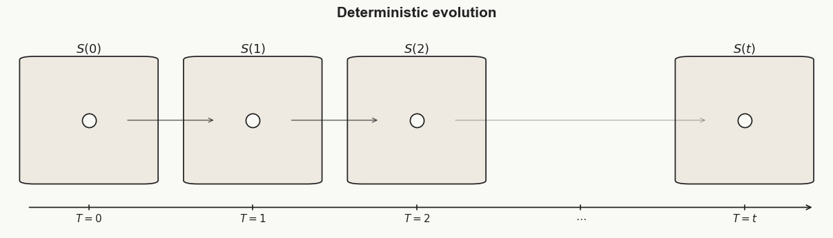
We can see this through a simple deterministic scenario. Consider a ball rolling down a hill from a fixed starting point. We can encode the initial conditions, such as the x-, y-, and z-coordinates of the ball and its initial velocity, along with the relevant laws of motion, using a constant number of bits, C. Now, to generate a specific state of this system, say at time T, we only need to encode the time step of that state. Starting from t = 0, we can use the encoded information to compute the state at t = T. Therefore, the Kolmogorov complexity of this system at time T is at most C + log(T) bits.
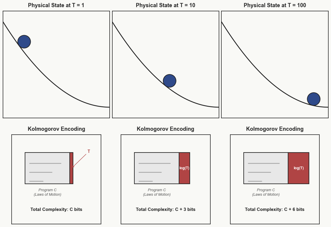
We notice that as the time step increases, the additional information required to describe the system grows only logarithmically. This is much slower than the growth we might expect from disorder spreading through the system, because we are using the laws of motion to compute the state rather than encoding it directly. To put it in perspective, apart from a constant C bits of information, encoding the age of the universe in seconds would require only about 59 bits.
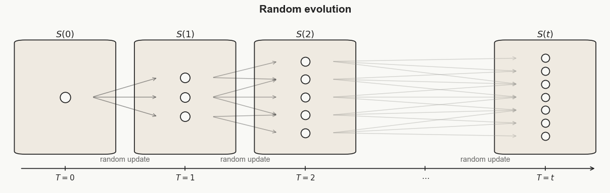
Aaronson quickly points out that while this idea is good for reconstructing a system, it fails to capture the system's apparent growing disorder. To address this, he proposes two solutions. His first solution is to consider a system with new randomness at each step, rather than a fixed deterministic one. This would force the random variables to be encoded with each time step, greatly increasing the information required to describe the system's evolving state.
One example could be encoding a game of pool where a coin toss determines whether I aim at a striped or solid ball. Assuming the initial setup and laws of motion are encoded in a constant number of bits C, each time step would also require storing the outcome of the coin toss. In the simplest case, this makes the Kolmogorov complexity grow linearly with time; if the number of random variables introduced at each step itself grows with time, this growth can become polynomial.
The other solution Aaronson proposes is to constrain the computation time available to the program. As we mentioned above, at every step, the state is being recomputed from the laws and initial conditions rather than decoded from stored information. In a step-by-step simulation, this means that to generate the state of the system at time T, the program may need to compute all previous states up to time T − 1. This quickly becomes impractical, because the time needed to reconstruct the state grows with T: the further ahead you want to generate, the longer you have to wait. Therefore, by placing a restriction on running time, we force the program to encode more of the system’s intermediate information directly, driving the Kolmogorov complexity up again.
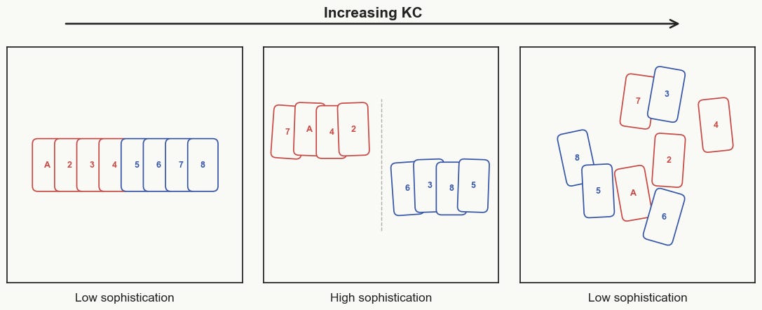
With this, Aaronson shows how Kolmogorov complexity can begin to track the growing disorder of a system, either by introducing randomness or by placing limits on computation time. This makes it a useful first attempt at giving our intuitive idea of complextropy a formal, quantitative footing, since it seems to capture the difference between order and disorder quite naturally. A sorted deck of cards can be generated with a simple rule, while a completely shuffled deck requires far more information to reproduce exactly. Even a partly structured deck, say one where the face cards and number cards are grouped in some pattern, would sit somewhere in between.
But this immediately creates a problem. In terms of raw Kolmogorov complexity, K(x), a typical randomly shuffled deck will typically have a high value because no short program can reproduce that exact arrangement of cards. And yet, intuitively, it still feels like one of the least complex things imaginable. We can describe its character very easily by saying, “It is random.” This raises the real question Aaronson is trying to get at: how do we capture complextropy as more than just the information needed to reproduce a state?
The answer lies in shifting our focus from the state itself to the structure behind it. This is where Aaronson brings in the idea of sophistication. Instead of asking only how much information is needed to describe a state, sophistication asks how much information is needed to describe the structure that could have produced it. To make this shift precise, we stop looking at x in isolation and instead look at the groups it could belong to.
Mathematically, we begin with a set S of n-bit strings, and a state x that belongs to it. The reason we can speak this way is that any state we care about, such as a particular arrangement of cards in a deck, can be encoded as a string. K(S) is the length of the shortest program that can describe or generate the set S, while K(x|S) is the length of the shortest program that can output x once S is already known. Intuitively, S is the category or explanation we place x inside, and K(x|S) is the extra information needed to pick out x from within that category.
For example, let x be the exact middle arrangement shown below: the red cards are grouped, the blue cards are grouped, but the cards inside each group are still shuffled. One possible set S could be “all decks where red and blue cards are separated.” The cost of describing this rule is K(S). This set is easy enough to describe, and the arrangement shown does not stand out within it. But S only tells us the broad structure of the arrangement, not the exact arrangement itself. Many decks could have red and blue cards separated while still having a different order within each group. To identify x specifically, we still need to know the order of the red cards and the order of the blue cards inside the two groups. This remaining information is K(x|S): the cost of picking out x once S is already known.
With this example in mind, we can now define sophistication more directly. The sophistication of x, written as Soph(x), is the smallest possible value of K(S) over all sets S where two things are true: x belongs to S, and x does not stand out inside S. In simpler terms, Soph(x) asks us to search across all possible categories that x could belong to, and pick the easiest-to-describe one where x still looks “ordinary”.
But what does it mean for x to look ordinary inside S? And why does that matter? Intuitively, x is ordinary inside S if it does not have some special shortcut that makes it easier to identify than a typical member of S. In the card example, if S is “all possible deck arrangements,” then our middle arrangement is not really ordinary inside it, because it has an obvious structure: the red and blue cards are separated.
This matters because without this condition, the definition can collapse. If we only searched for the easiest-to-describe set containing x, we could always choose something extremely broad, like “all possible deck arrangements.” That set has a small K(S), so our middle arrangement would incorrectly appear to have low sophistication. The genericity condition prevents this shortcut. It forces us to choose a set where x actually looks ordinary, not just one where x technically belongs.
Mathematically, this is captured by K(x | S) ≥ log(|S|) − c. If S has |S| possible elements, then identifying a typical element inside S should take roughly log(|S|) bits, with c giving us a small amount of slack. But if x can be picked out using far fewer bits, then x is not really ordinary inside S. This is why sophistication is not just looking for the simplest category, but the simplest category where x does not become an exception. And since S does not have to be written out as a massive list, we can think of it as a rule or condition that decides membership, like “all deck arrangements where red and blue cards are separated.” So when we ask whether x belongs to S, we are really asking whether x passes this membership test.
Now, how does this help us? After this heavy exercise, Aaronson points out that sophistication has the behaviour we originally wanted from complextropy: it is low for simple states, low again for uniformly random states, and high for states that are neither fully simple nor fully random, but somewhere in the middle.
However, we now run into a familiar problem. In a deterministic system with fixed initial conditions, the set of possible states at time t, S(t), contains only one state, because the system has only one expected outcome after t steps. So S(t) can still be described very cheaply: we only need the initial conditions, the rules of evolution, and the time t. This means K(S(t)) grows no faster than log(t) + c. Since Soph(x) is defined by minimising K(S) over all valid sets S, Soph(x) also cannot grow faster than this logarithmic bound.
Introducing randomness seems like a possible fix, because now there are many possible states at time t, not just one. But even here, sophistication remains too cheap. To describe one specific randomly generated state x, we would need to encode the particular random choices that led to it. But S(t) contains all possible states the system could reach at time t, so we do not need to store each outcome separately. We only need the initial conditions, the rule for how randomness enters the system, and the time t. The rule generates the whole set for us. So even after introducing randomness, K(S(t)) still grows only logarithmically, and in turn, so does Soph(x). Randomness gives us many possible states, but it does not make the set of those states hard enough to describe.
Hence, as we did before with Kolmogorov complexity, we constrain the computation time available to the program. Now, the program cannot just give a short description of S and take forever to generate it. It has to describe S efficiently. This forces more of the system’s structure to be encoded directly, allowing sophistication to escape the logarithmic bound we kept running into.
However, this also means the membership test needs to be constrained. If the test has unlimited time, it could keep searching for some extremely hidden property that makes even a generic-looking x easier to identify. That would weaken the whole idea of genericity, because x would no longer be ordinary inside S. So, just like the program describing S, the membership test also has to run within a bounded time.
With both constraints in place, sophistication becomes resource-bounded sophistication. Instead of asking for the shortest program that describes a set S where x is generic, we now ask for the shortest efficient program that describes such a set, under an efficient membership test. This gives us the version of sophistication needed to get closer to complextropy: low for simple and fully random states, but large somewhere in the middle.
The Point
So why did we go through all of this?
We started with complextropy: the intuition that complexity is low for pure order, low for pure randomness, and high somewhere in the middle. But the moment we tried to make this precise, the obvious measures began to break. Plain Kolmogorov complexity made randomness look maximally complex. Sophistication helped by shifting our attention from the state itself to the structure that could have produced it, but even that was not enough. Without limits on computation, the structure behind a system could still be described too cheaply. This is why resource-bounded sophistication matters: it gets closer to the kind of complexity we were pointing at all along, not just disorder, and not just structure, but structure that is non-trivial to find, describe, or generate under limited resources.
This is also where the connection to learning becomes clearer. Learning is not just about storing more information; it is about finding useful structure in that information. A model tries to do something similar: discover a representation where examples stop looking like isolated data points and start looking like members of a category or pattern it can use. Sophistication, and in turn, complextropy, tells us where this becomes interesting. Pure order is too simple. Pure randomness gives us nothing to learn. The middle is where structure exists, but still has to be discovered.
In some sense, this is also how machine learning has evolved: finding better and better ways to represent that messy middle. From simple mathematical models to deep neural networks, the goal has remained strangely familiar: find the tightest structure in which the data stops looking random and starts making sense. That is why this article feels like the right starting point for this series. Before jumping into models, architectures, and implementations, it's worth starting with the deeper question underlying them all: what does it even mean for something to have structure?
So here’s to complextropy: the kind of complexity that peaks in the middle. The universe is not just a hot ball of plasma at the beginning or cold, dead nothing at the end. It is the messy middle filled with galaxies, stars, planets, and eventually, you and me.
Thank you for sticking till the end. I hope you enjoyed this!
References
For the main thread of this series and all related posts, check out SUT30-000.
So interesting! Love how you broke down the concepts